Automated De Novo Protein Design Optimization
De novo protein design has advanced rapidly through generative models: diffusion-based structure generators (Proteina-Complexa, RFdiffusion), structure predictors (AlphaFold2, RoseTTAFold3), conformational samplers (BioEmu), and inverse folding networks (ProteinMPNN, LigandMPNN). These models are powerful. But using them to produce high-quality binders for a specific target requires searching over dozens of inference-time hyperparameters: beam search width, checkpoint schedules, branching factors, scoring model choice, refinement strategies, and more. No single default configuration works across targets. The search is high-dimensional, target-dependent, and expensive.
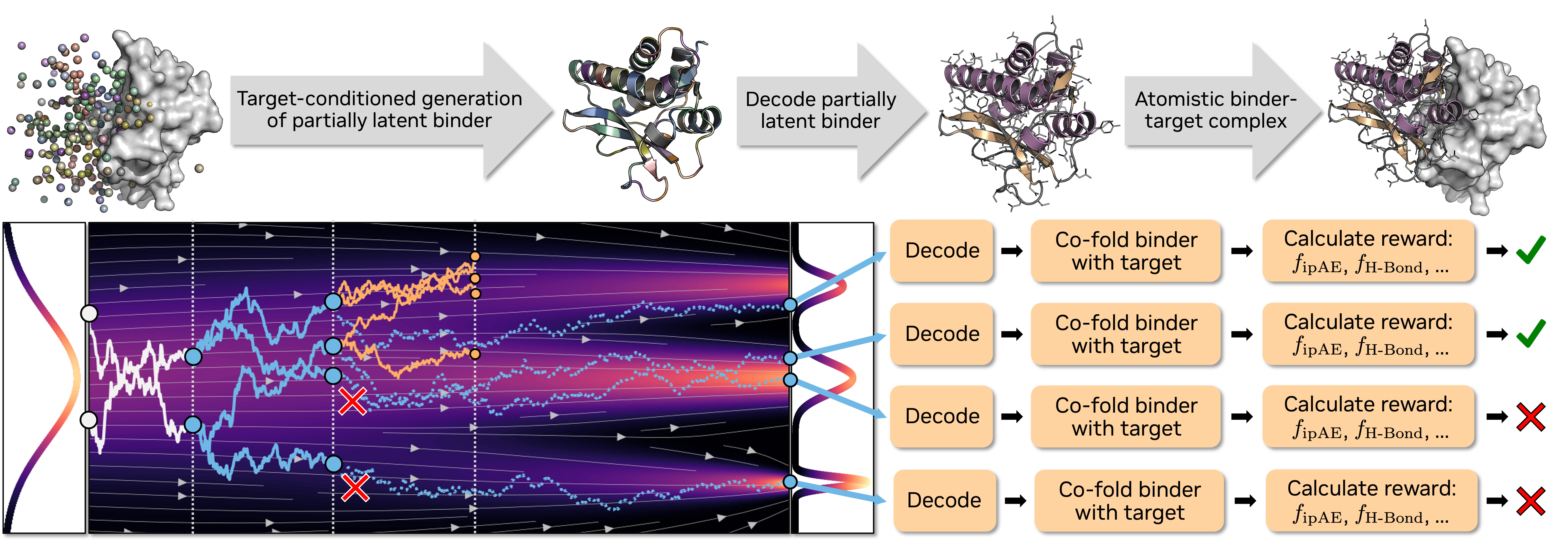
We frame this as an inference-time optimization problem. The trained model weights are fixed. The agent's job is to find the best way to run the model for each target. LLMs can act as the brain that connects to and orchestrates protein design models, turning what was a manual trial-and-error process into a closed-loop optimization.
Can an LLM agent optimize inference-time hyperparameters for protein generative models, improving binder quality iteration by iteration for each target?
Four generations of the agent, laid out by what the LLM actually writes and whether it reasons about one protein or a whole protein set at once. v3 and v4 both evolve an inference program — the difference is scope.
orchestrator.py that decides, within a step+wallclock budget, how to spend compute across N targets (reorder, batch, skip, retry) — all per-target inference still flows through the host-sanctioned run_single_target(ctx, target) chokepoint, so the LLM owns the policy while the host owns the subprocess boundary.The agent minimizes i_PAE (binding quality) while maintaining high pLDDT (fold confidence). Example on the CD45 target (hardest, largest improvement):
Motivation: Good Models Need Good Hyperparameters
We ran 50 experiments (5 beam search configs × 10 protein targets) with Proteina-Complexa. The results make the case clearly:
E_fine_selector wins 7/10, but D_early_brancher wins IFNAR2, C_deep_exploiter wins PD-L1. The #1 config varies per target.
4/10 proteins have different optimal configs depending on whether you pick top-1 or pool top-16 candidates.
BetV1 (CV=0.65): config choice changes reward by 50%. IFNAR2 (CV=0.03): any config works.
Different search strategies produce different sequences. Multi-config pooling beats single-config compute.
Motivation 2: The Full Inference-Time Control Surface
The challenge goes beyond tuning scalar hyperparameters. A generative pipeline like Proteina-Complexa exposes 80+ inference-time parameters organized across qualitatively different layers:
Which algorithm to use (beam search, MCTS, FK-steering, best-of-n), how to branch, when to prune, at which checkpoints.
How many steps, noise schedules, guidance weights, self-conditioning, ODE integration limits. These controls shape how the generative model samples.
Which scoring model (AF2, RF3, Boltz2), which metrics to optimize (i_PAE, pLDDT, i_con, radius of gyration), how to weight them.
Whether to enable sequence hallucination, ProteinMPNN redesign, or LigandMPNN; self-consistency checks; structural filters.
Composing cheap exploration → expensive refinement; conditional compute allocation; re-ranking under alternative criteria.
These are not parameters to grid-search. They are design decisions that require reasoning about the target, the failure mode, and the experimental goal. This is why LLM agents, rather than Bayesian optimization alone, are the right tool: they can reason about which knobs to turn, not just how far.
Why the Control Surface Is So Large: Branching Inside Flow Matching
Proteina-Complexa generates structures via conditional flow matching, a learned velocity field that denoises Gaussian noise into protein structure over T steps. The key architectural feature is partial simulation: the denoising loop can pause at intermediate checkpoints, return the state, and let search algorithms branch, evaluate, and prune within a single generation run:
step_checkpoints = [0, 100, 200, 300, 400]

Checkpoint 0 (pure noise):
  Initialize beam_width × nsamples noise samples

  ── Denoise steps 0 → 100 (partial simulation) ──

Checkpoint 100:
  BRANCH: duplicate each beam into n_branch copies
  LOOKAHEAD: roll out each copy to step 400 (completion)
  SCORE: evaluate i_PAE on completed structures
  SELECT: keep top beam_width candidates per sample

  ── Continue denoising 100 → 200 with selected beams ──

Checkpoint 200:
  BRANCH → LOOKAHEAD → SCORE → SELECT

  ...repeat at each checkpoint until step 400 (final)
Four search algorithms exploit this differently: beam search (branch, lookahead-score, keep top-k), best-of-N (independent full trajectories, pick best), FK-steering (branch + steer with reward signal + temperature), and MCTS (PUCT tree search over checkpoint branches).
This is what makes the optimization surface deeply coupled rather than flat:
- Where to branch (checkpoint placement): correcting early structural decisions vs. late refinements
- How to branch (n_branch, noise injection): diversity vs. exploitation of promising intermediates
- How to score (reward weights, AF2 recycles): what the lookahead evaluations actually measure
- How to denoise (ODE vs. SDE, schedule shape, guidance): the character of each trajectory segment
- How to chain stages (cheap explore → conditional refine): compute allocation based on intermediate evidence
These decisions interact: checkpoint placement only matters given a particular denoising mode; reward weights only matter given a particular branching strategy. This is why we frame the problem as composing InferencePrograms rather than tuning flat hyperparameters. The decisions form a structured, multi-level control program over the generation process. (See Pipeline Details below for the full technical breakdown.)
We formalize this as inference-time scaling: the LLM agent does not change the trained model backbone or weights. Instead, it learns to compose multi-stage InferencePrograms: executable plans that specify search policy, sampling controls, reward weighting, refinement strategy, and conditional transitions between stages. The agent evolves these programs through population-based search, treating each experiment as an evolvable artifact with lineage tracking and duplicate detection.
A human researcher running Proteina-Complexa on a new drug target faces a combinatorial space: 5 search algorithms × checkpoint schedules × branching factors × reward compositions × refinement strategies × multi-stage sequencing. This is not a hyperparameter grid. It is a space of programs. Running all combinations for every target is infeasible. An LLM agent that understands the target–config interaction can adaptively allocate compute: scouting cheaply first, then investing in promising strategies, composing multi-stage programs, and transferring learnings across targets.
Pipeline Details: Proteina-Complexa
[Target PDB + Hotspots] → Flow Matching (400 steps) → Beam Search → AF2 Scoring → Candidate PDBs| Stage | What it does | Key hyperparameters |
|---|---|---|
| Generate | Flow-matching diffusion in partially latent space | nsteps, guidance_w, self_cond |
| Search | Beam search with branching at checkpoints | beam_width, n_branch, checkpoint schedule, nsamples |
| Score | AF2 multimer reward (i_PAE) | num_recycles, reward weights |
| Refine | Sequence hallucination (test-time optimization) | n_iters, loss weights, temperature |
Hardware: 8× NVIDIA H100 80GB | Targets: 44 pre-configured (10 proteins + 4 ligand targets used in sweeps) | Scale: 26,560 samples from 50 protein binder experiments
Flow Matching: Technical Details
The generative model uses conditional flow matching in a product space of two data modes, each with independent schedules and noise injection:
| Mode | What it represents | Dimension |
|---|---|---|
| bb_ca | Backbone Cα coordinates | [n_residues, 3] |
| local_latents | Compressed local structure (via autoencoder) | [n_residues, latent_dim] |
At each step, the neural network predicts the clean structure x̂ from the current noisy state xt. The update rule depends on the sampling mode:
| Mode | Update rule | Character |
|---|---|---|
vf | x ← x + v·dt | Pure ODE: deterministic, low variance |
sc | x ← x + (v + g(t)·s)·dt + noise | SDE: stochastic, higher diversity |
vf_ss | Score-scaled ODE with temperature control | Temperature-tuned deterministic |
vf_tsr | SNR-based adaptive temperature scheduling | Advanced adaptive |
Each mode has its own time schedule (how to partition [0,1] into steps: log, power, uniform, cosine), noise injection schedule g(t) (1/t, tangent, power-law variants), and step parameters (noise scale, score scale, ODE/SDE switching thresholds). Optional self-conditioning feeds back the previous step’s prediction, and classifier-free guidance or auto-guidance can steer generation toward the conditioning target.
Evidence: Sweep Results and Per-Protein Optimality (50 experiments)
Beam Search Sweep Rankings
| Rank | Config | Strategy | Mean Reward | Wins (top-1) |
|---|---|---|---|---|
| 1 | E_fine_selector | 6 checkpoints, 3 branches | −0.2475 | 7/10 |
| 2 | A_balanced | Paper default | −0.2571 | 0/10 |
| 3 | C_deep_exploiter | 2 lengths, 16 beams | −0.2700 | 1/10 |
| 4 | D_early_brancher | 8 branches, 2 checkpoints | −0.2792 | 2/10 |
| 5 | B_length_explorer | 16 lengths, 2 beams | −0.3501 | 0/10 |
The gap between best and worst config (0.103 mean reward) is ~42% relative difference. For hard targets like BetV1, the gap is even larger. Choosing the right hyperparameters matters as much as choosing the right model.
Per-Protein Optimality
The optimal config depends on both the target and what you optimize for:
| Protein | Top-1 Winner | Top-16 Pool Winner | Same? |
|---|---|---|---|
| CD45 | E_fine | A_balanced | NO |
| Claudin-1 | D_early | E_fine | NO |
| DerF7 | D_early | E_fine | NO |
| SpCas9 | E_fine | C_deep | NO |
| 6 other proteins: same winner for both criteria | |||
This is exactly the kind of problem LLM agents can solve: high-dimensional configuration spaces, target-dependent optima, and multi-objective trade-offs.
Model Landscape: 6 Models in the Agent Framework
The agent framework is designed to work across multiple protein and molecular models:
| Model | Type | What it does | Status |
|---|---|---|---|
| Proteina-Complexa | Binder Design | Flow-matching de novo binder generation with beam search (protein + ligand binder modes) | Active: 50 protein + 20 ligand experiments |
| AlphaFold2 | Scoring | Structure prediction & binding quality assessment (i_PAE, pLDDT) for protein targets | Active: reward model for protein binders |
| RoseTTAFold3 | Scoring | Structure prediction for protein–ligand complexes (min_ipAE, ipTM) | Active: reward model for ligand binders |
| ProteinMPNN | Inverse Folding | Sequence redesign for designability evaluation (scRMSD) | Active: enabled in ligand binder evaluation |
| LigandMPNN | Ligand-Aware Design | Ligand-aware sequence redesign for small-molecule binders | Active: in ligand binder evaluation |
| BioEmu | Dynamics | Protein conformational ensembles, 1000s of structures/hour/GPU. Predicts folding stability (ΔG), captures domain motion & local unfolding | Planned: assess binder robustness to target flexibility |
BioEmu (Microsoft Research, Science 2025) generates conformational ensembles 10,000–100,000× faster than molecular dynamics. A designed binder must work not just against the crystal structure, but across the target's dynamic conformations. BioEmu can generate these ensembles in minutes, enabling the agent to test binder robustness as part of the design loop.
Models: Proteina-Complexa · BioEmu (Science 2025) · ProteinMPNN
Related: Tinker Explorer: RL agent for budget-constrained sequential decisions (parallel theme: adaptive compute allocation under step budgets)
Pipeline Validation: PD-L1 Binder Demo
Validate the Proteina-Complexa pipeline end-to-end: can we generate protein binder candidates and score them with AlphaFold2 on our hardware?
First run: PD-L1 target (Programmed Death-Ligand 1), 100 diffusion steps, 2 samples, best-of-n search with 1 replica. Deliberately minimal to test the pipeline, not the quality.
Results
| Metric | Sample 0 (n=262) | Sample 1 (n=234) |
|---|---|---|
| total_reward | −0.831 | −0.881 |
| i_PAE | 0.831 | 0.881 |
| pLDDT | 0.212 | 0.239 |
| RMSD | 11.25 Å | 45.21 Å |
82.92 seconds total on 1× H100 (41.5s per sample). Pipeline functional.
Quality Thresholds (Demo vs Production)
Both samples fail production thresholds. Expected at 100 steps with no refinement:
| Criterion | Demo Result | Threshold | Status |
|---|---|---|---|
| i_PAE × 31 ≤ 7.0 | 25.76 / 27.32 | ≤ 7.0 | FAIL |
| pLDDT ≥ 0.9 | 0.212 / 0.239 | ≥ 0.9 | FAIL |
Pipeline works. Quality requires production settings: 400 steps, more samples, beam search, and refinement. Full report →
Beam Search Configuration Sweep (5 configs × 10 proteins)
How do different beam search strategies (varying checkpoint frequency, branching factor, and length sampling) affect binder quality across diverse protein targets?
5 Beam Search Configurations
All configs use 400 diffusion steps and produce 32 final PDBs per experiment. They differ in how they allocate compute during search:
| Config | nsamples | beam_width | n_branch | Checkpoints | Strategy |
|---|---|---|---|---|---|
| A_balanced | 4 | 8 | 4 | [0, 100, 200, 300, 400] | Paper default |
| B_length_explorer | 16 | 2 | 4 | [0, 100, 200, 300, 400] | Max length diversity |
| C_deep_exploiter | 2 | 16 | 4 | [0, 100, 250, 400] | Deep per-length optimization |
| D_early_brancher | 4 | 8 | 8 | [0, 200, 400] | Wide early exploration |
| E_fine_selector | 4 | 8 | 3 | [0, 65, 130, 200, 270, 340, 400] | Frequent fine-grained pruning |
10 protein targets: PD-1, PD-L1, IFNAR2, CD45, Claudin-1, CrSAS-6, DerF7, BetV1, SpCas9, HER2
Scale: 50 experiments × 8 GPUs = ~93 min runtime. 26,560 total samples (1,600 finals).
Final Rankings (50 of 50 Complete)
| Rank | Config | Mean Reward | Best i_PAE | Mean pLDDT |
|---|---|---|---|---|
| 1 | E_fine_selector | −0.2475 | 0.137 | 0.076 |
| 2 | A_balanced | −0.2571 | 0.133 | 0.095 |
| 3 | C_deep_exploiter | −0.2700 | 0.141 | 0.093 |
| 4 | D_early_brancher | −0.2792 | 0.130 | 0.094 |
| 5 | B_length_explorer | −0.3501 | 0.136 | 0.112 |
D_early_brancher initially appeared #1 (mean −0.2119) when only 4/10 proteins had completed, all easy targets. With full data, it drops to #4. Partial results can mislead.
Protein Difficulty Ranking
| Difficulty | Protein | Best i_PAE | Best Config |
|---|---|---|---|
| Easy | IFNAR2 | 0.130 | D_early_brancher |
| Easy | PD-1 | 0.138 | E_fine_selector |
| Easy | PD-L1 | 0.150 | C_deep_exploiter |
| Easy | CrSAS-6 | 0.156 | E_fine_selector |
| Medium | CD45 | 0.159 | E_fine_selector |
| Medium | SpCas9 | 0.168 | E_fine_selector |
| Medium | DerF7 | 0.175 | E_fine_selector |
| Medium | Claudin-1 | 0.193 | D_early_brancher |
| Hard | BetV1 | 0.205 | E_fine_selector |
| Hard | HER2 | 0.222 | E_fine_selector |
Config Diversity: Per-Protein Optimality & Sequence Space
The optimal beam search configuration is protein-dependent. The winner changes depending on both the target and the selection criterion (top-1 vs top-16 pool). Different configs explore different regions of sequence space.
Full Per-Protein Config Ranking (10 × 5)
Ranking each config 1–5 per protein reveals that no config is universally best or worst. The #1 position is held by 3 different configs across the 10 proteins:
| Protein | #1 (Best) | #2 | #3 | #4 | #5 (Worst) |
|---|---|---|---|---|---|
| PD-1 | E_fine | A_bal | B_len | D_early | C_deep |
| PD-L1 | C_deep | E_fine | A_bal | D_early | B_len |
| IFNAR2 | D_early | A_bal | E_fine | B_len | C_deep |
| CD45 | E_fine | A_bal | C_deep | D_early | B_len |
| Claudin-1 | D_early | C_deep | A_bal | E_fine | B_len |
| CrSAS-6 | E_fine* | D_early* | B_len | A_bal | C_deep |
| DerF7 | D_early* | E_fine* | C_deep | B_len | A_bal |
| BetV1 | E_fine* | D_early* | B_len | A_bal | C_deep |
| SpCas9 | E_fine | C_deep | D_early | A_bal | B_len |
| HER2 | E_fine | A_bal | B_len | C_deep | D_early |
* Near-ties (< 0.001 difference), effectively equivalent, winner depends on random seed.
Top-1 vs Top-16: The Winner Changes
When switching from “which config finds the single best binder?” to “which config produces the best pool of 16 candidates?”, the winner changes for 4 out of 10 proteins:
| Protein | Top-1 Winner | Top-16 Pool Winner | Same? |
|---|---|---|---|
| CD45 | E_fine | A_balanced | NO |
| Claudin-1 | D_early | E_fine | NO |
| DerF7 | D_early | E_fine | NO |
| SpCas9 | E_fine | C_deep | NO |
| PD-1 | E_fine | E_fine | Yes |
| PD-L1 | C_deep | C_deep | Yes |
| IFNAR2 | D_early | D_early | Yes |
| CrSAS-6 | E_fine | E_fine | Yes |
| BetV1 | E_fine | E_fine | Yes |
| HER2 | E_fine | E_fine | Yes |
If you plan to experimentally test 16 candidates, optimizing for top-1 gives you the wrong config for 40% of targets. The selection criterion must match the experimental plan.
Sequence Diversity
Beyond finding different quality binders, configs generate structurally and sequentially distinct candidates:
- Length distributions differ: B_length_explorer samples 16 binder lengths (broadest); C_deep_exploiter samples only 2 (narrowest). Same target, very different structural coverage.
- Inter-config sequence identity is lower than intra-config: Sequences from different configs share less identity than sequences within the same config. The search strategies explore different regions of the design landscape.
- Amino acid composition varies subtly: Different configs show 2–5% differences in hydrophobic/polar/charged residue fractions, reflecting different design biases.
Practical Implications
| Your Goal | Recommendation |
|---|---|
| Test 1 candidate | Use E_fine_selector (wins 6–7/10 proteins) |
| Test 16 candidates | Check the per-protein winner (it varies) |
| Hard target (high CV) | Run 2–3 configs and pool. Config choice is critical |
| Easy target (low CV) | Any config works. Save compute |
| Maximize diversity | Multi-config pooling. Different configs = different sequences |
Agent Loop v1: Closed-Loop Hyperparameter Search
Can an LLM agent autonomously improve binder quality by iteratively selecting configurations, running experiments, analyzing results, and adapting its strategy?
Optimization Trajectories
Each target shows a clear improvement trajectory. The agent achieves 10–28% improvement in best i_PAE from baseline:
| Target | Runs | Start i_PAE | Best i_PAE | Improvement | Best Config |
|---|---|---|---|---|---|
| PD-1 | 4 | 0.166 | 0.133 | -20% | bw=8, nb=4, ns=8, fine ckpts |
| PD-L1 | 8 | 0.158 | 0.134 | -15% | bw=16, nb=4, ns=4, fine ckpts |
| IFNAR2 | 5 | 0.145 | 0.130 | -10% | bw=16, nb=8, ns=4, standard ckpts |
| CD45 | 4 | 0.241 | 0.173 | -28% | bw=16, nb=4, ns=4, standard ckpts |
Per-Target Trajectory Detail: Run-by-Run Logs
Run 1: bw=8,nb=4,ns=4,standard → 0.166
Run 2: bw=8,nb=4,ns=4,fine → 0.138 (-17%)
Run 3: bw=8,nb=4,ns=8,fine → 0.133 (-20%)
Run 4: mcts,bw=8,nb=4,ns=8 → 0.138 (regressed)
Run 1-3: bw=8,nb=4,ns=4 → 0.158 (3 duplicates)
Run 4: bw=8,nb=4,ns=8 → 0.156
Run 5: bw=16,nb=4,ns=4 → 0.165 (worse)
Run 6: bw=8,nb=4,fine → 0.150
Run 7: bw=16,nb=4,fine → 0.134 (-15%)
Run 8: bw=16,nb=8,fine → OOM
Run 1: bw=8,nb=4,ns=4 → 0.145
Run 2: bw=16,nb=4,ns=4 → 0.139
Run 3: bw=16,nb=8,ns=4 → 0.130 (-10%)
Run 4: mcts,bw=16,nb=8 → 0.146 (regressed)
Run 5: bw=16,nb=8,ns=8 → 0.133
Run 1: bw=8,nb=4,ns=4 → 0.241
Run 2: bw=8,nb=4,fine → 0.180 (-25%)
Run 3: bw=8,nb=4,ns=8,fine → 0.180
Run 4: bw=16,nb=4,fine → 0.173 (-28%)
Key Findings from 21 Runs
Switching from standard (5-point) to fine-grained (7-point) checkpoints produced the largest single improvement for PD-1 (-17%) and CD45 (-25%).
Tried on PD-1 and IFNAR2, both times regressed. Beam search with larger beam_width consistently outperformed.
PD-L1's best config (fine ckpts + bw=16) combined two changes. The "change one variable at a time" instruction prevented discovering this earlier.
The agent launched identical PD-L1 configs 3 times in one session: no deduplication, no history check. A BO method would never do this.
v1 Results and Reflection
The agent achieves 10-28% improvement on every target, but the search strategy has clear limitations:
Same 4 knobs in the same order for every target. Never tried fk-steering, best-of-n, or nsteps<400. A GP-BO would likely match results in ~10 runs vs 21. No surrogate model, no transfer across targets.
Best i_PAE (0.130–0.134) is marginal vs BindCraft validated threshold (<0.10). pLDDT is excellent (0.94–0.96). CD45 fails due to only 1 hotspot residue. ProteinMPNN is disabled. Enabling it is the single highest-impact change.
GPU utilization ~35–40%. 25% compute wasted on 3 duplicate PD-L1 runs. No auto-retry on OOM, no file locking for concurrent agents. Total cost: ~16 GPU-hours ($47).
Full interactive dashboard with per-run details and Plotly visualizations →
v2 Plan: From Configs to Programs
v2 was the transitional design that introduced tree search and InferenceProgram as the unit of evolution. The active track is now v3 below, which keeps v2's tree-search core but makes research ideas first-class alongside the programs themselves, explicitly following the SCORE decomposition.
v1 showed that the agent loop works and that how you spend compute matters more than how much. The question for v2: what if the agent could compose programs instead of picking configs?
What is the right abstraction for inference-time computation in generative protein design, and can an LLM reason about it?
The agent currently picks from 5 named presets differing in 4 knobs. But the real design space is 80+ parameters across 6 qualitatively different layers (search, sampling, reward, refinement, filtering, orchestration), and the interesting choices are conditional: "refine only if i_PAE < 0.25", "switch scoring model based on target type", "double beam width if early steps show high variance." These are not hyperparameters. They are programs.
Can LLM-guided program evolution outperform Bayesian optimization in structured, high-dimensional spaces where the search objects are programs, not vectors?
The v1 agent uses the same 4 knobs in the same order for every target, with no memory across sessions. A population of programs with lineage tracking, crossover, and deduplication turns the agent from a sequential optimizer into an evolutionary researcher that builds on its own history.
Is there an inference-time scaling law for protein design, and can an LLM agent find it?
v1 showed that E_fine_selector beats B_length_explorer by 42% with the same GPU budget. v2 tests a stronger claim: that an agent composing multi-stage programs (scout → invest → pool) can turn additional compute into monotonically better designs, the way test-time compute scaling works for LLM reasoning.
Experiment: Graphify for Codebase Understanding
A key bottleneck for the agent is understanding the Proteina-Complexa codebase well enough to reason about which parameters exist, how they interact, and what new configurations are possible. The codebase has thousands of lines of Hydra configs, model definitions, and pipeline scripts. Reading these files sequentially is slow and loses structural relationships.
We will test whether Graphify, a tool that converts code, documentation, and configs into a knowledge graph with clustered communities, can help. The idea:
Run Graphify on the Proteina-Complexa codebase: Hydra configs, model classes, pipeline scripts, scoring modules. Extract entities (parameters, functions, config groups) and relationships (parameter → affects → pipeline stage).
When the agent decides which parameter to try next, it queries the knowledge graph instead of reading raw files. "What parameters affect beam search scoring?" returns a structured subgraph, not thousands of lines of code.
Compare agent performance with and without the graphified knowledge base: does it discover more of the 80+ parameter space? Does it avoid duplicate runs? Does it find better configs in fewer iterations?
The graphified knowledge base will help the agent discover parameters it currently ignores (noise schedules, guidance weights, sampling modes, refinement settings) and reason about parameter interactions that are invisible when reading configs sequentially.
Orthogonal Experiments Backlog
Items about program representation, deduplication, 80+ parameter surface, population-based search, and LLM-vs-BO benchmarking have moved to v3, which now owns them. What remains here is the orthogonal experiment backlog — work that is not about the agent loop itself but about the downstream pipeline, conformational robustness, scoring models, and codebase tooling.
| Priority | Task | Status |
|---|---|---|
| P0 | Enable ProteinMPNN redesign + scRMSD filter in protein binder pipeline (identified as single highest-impact change in v1 reflection) | Pending |
| P0 | Complete ligand binder sweep: 18/20 experiments remaining (configs B-E for all 4 ligand targets) | In progress |
| P1 | Run Graphify on Proteina-Complexa codebase: build knowledge graph, evaluate whether it improves the mutator's ability to find uncovered parameters | Pending |
| P2 | Integrate BioEmu for conformational ensemble robustness testing | Pending |
| P2 | Cross-model orchestration: agent selects AF2 vs RF3 vs Boltz2 scoring per target | Pending |
v3: From Programs to Ideas + Programs
v2 asked: what if the agent composes programs instead of picking configs? v3 asks a tighter question: what if the agent also evolves the scientific ideas behind those programs, and the search tree knows about both? v3 is an explicit implementation of the SCORE decomposition (Aygun et al. 2025), narrowed to Proteina-Complexa inference-time binder design.
AutoresearchV3 = ScorableTask + ResearchIdeaLibrary + LLM Mutator + Sandbox Executor + Tree Search + Fixed Evaluator
The Six Primitives
The v3 loop makes every SCORE primitive a first-class host object. Each expansion step touches all six:
ChildProposals that must clear validation before hitting the sandbox. The dashed feedback edge is the SCORE outer loop — tree search picks which (idea, program) node to expand next.Research Ideas as First-Class Objects
The most important conceptual shift from v2 is that a ResearchIdea is not code, not a program, and not a prompt fragment. It is a persisted, hashable, recombinable hypothesis object with its own lineage. Every program in the tree points back to one or more ideas, and mutations are typed by what they do to those ideas.
ResearchIdea:
  idea_id
  title
  summary
  hypothesis
  implementation_hints
  source_type  # user|llm|paper|recombination
  parent_idea_ids
tags- diversify early with wider branching, exploit late with aggressive reranking
- use AF2 confidence + interface compactness as a secondary reranker
- replace hard top-k beam selection with stochastic temperature-weighted selection
- warm-start from high-confidence partial trajectories
Mutations are typed by their effect on the idea set, not just the code:
- idea_preserving
- idea_refining
- idea_branching
- idea_recombination
- module_synthesis / module_edit
- program_recombination
Without first-class ideas, an agent loop collapses into parent program → LLM prompt → child program. That misses the part of SCORE that makes it a research loop rather than a code-perturbation loop. Separating the idea from its implementation lets the tree reason about hypothesis diversity independently from code diversity, and lets two different programs that embody the same idea be recognized as such.
Content-Addressed Program Identity
Every persisted artifact in v3 has a content hash, and program identity folds the idea choice directly into the program:
spec_hash    = sha256(canonical(ProgramSpec \ {lineage_fields}))
bundle_hash  = sha256(canonical(CodeBundle))
program_hash = sha256(spec_hash + bundle_hash)
program_id   = program_hash[:12]

# selected_idea_ids ∈ spec_hash
# ⇒ picking different ideas yields a different program_id
# ⇒ the tree dedupes on (ideas + code), not code alone
This is what makes the joint search state above tractable: nodes are still program-centric for deduplication, but the expansion policy can reason about ideas separately because the idea choice is already baked into the identity.
Implementation Status
v3 lives at Autoresearch_Denovo/autoresearch_v3/ as a standalone package with its own Plan.md, ImplementationSpec.md, and pyproject.toml. Snapshot as of 2026-04-14 (verified by reading each module):
| Layer | Status | Detail |
|---|---|---|
| Artifacts & hashing | Done | ScorableTask, ResearchIdea, ProgramSpec, StageSpec, ModuleRef, CodeAsset, CodeBundle, ExecutableInferenceProgram, ProgramEvaluation — canonical JSON + content hashing, selected_idea_ids ∈ spec_hash |
Persistence (RunStoreV3 + IdeaBank) |
Done | atomic JSON writes for task / idea / asset / bundle / program / validation / evaluation / tree; check_duplicate gate |
| Host control surface | Done | SCHEMA_VERSION / VALIDATOR_VERSION / EVALUATOR_VERSION, allowed + banned import prefixes, patch whitelist, MAX_IDEAS_PER_PROGRAM |
| Validator (static) | Done | task + idea refs + program structure + AST parse + import allow/ban + patch format + patch whitelist + entry_symbol presence |
| Validator (runtime smoke) | Pending | Plan.md §9.2 step 8 — tiny import + instantiate check before real-run |
| Compiler | Done | ProgramSpec → normalized Hydra overrides + resolved module manifest (built-in refs + generated_reranker/etc. resolved against bundle assets) |
| Sandbox Executor | Dry-run verified | prepare_execution + run_single_stage (dry & real code paths). Real-run subprocess launches proteinfoundation.generate with sourced env.sh, CUDA_VISIBLE_DEVICES, and sandboxed PYTHONPATH. No recorded v3 GPU runs yet. |
| Evaluator (fixed) | Done | n_successful from reward CSVs: i_pae < 0.18 ∧ plddt_log > 0.90 ∧ sample_type == "final"; sequence-diversity diagnostic |
| Mutator (deterministic + LLM) | Done | propose_idea_branch, propose_param_mutation, propose_program_recombination, plus full LLM path: build_prompt_request → build_llm_prompts → parse_llm_proposal (strict JSON contract) → ChildProposal |
| LLM backend | Done | V1LLMClientAdapter (reuses v1's multi-provider client from autoresearch_common.llm) + StaticJSONClient for deterministic tests |
SearchDriver + CLI |
Done | initialize_task · run_single_step · run_n_steps; python -m autoresearch_v3 {init|step|loop} with --model / --static-payload / --real-run flags |
| Tree state | Done | TreeNode / TreeState: add_node, record_evaluation, best_nodes sort by (rank_key, mean_value), persistence to tree.json |
| Tree selection policy (PUCT / UCB) | Minimal | driver currently walks child-of-best; no UCB expansion yet — port from v2 plan pending |
| End-to-end dry-run | 2026-04-13 | full artifact chain persisted in _tmp_store_check/; compiled manifest in _tmp_exec_dryrun/exec_cd74ed879378/ — see below |
| Unit tests | 9 passing | tests/test_core.py: hash stability, validator, compiler ref resolution, mutator (branch / recombine / param), prompt builder, LLM proposal parse, end-to-end driver with dedup |
| Real GPU run of v3 on a target | Pending | dry-run entries exist in run_store/v3/ (5 tree nodes, 2 evaluated); first real GPU run blocked only by scheduling, not code |
| Multi-stage execution + warm-start | Pending | executor runs stage 0 only; Plan.md milestone 7 |
First end-to-end dry-run (2026-04-13)
The scratch dirs capture a real run of the full loop: host registers a ScorableTask for PD-L1, seeds an IdeaBank, the mutator (via StaticJSONClient) emits a ChildProposal with a generated reranker asset, the validator passes the program, the compiler resolves the module manifest, the executor materializes it into a sandbox, and the evaluator + tree record the result. This exercises every host object in the six-primitives diagram above.
generated_reranker:simple to the asset reranker_0b0ee075e9b3 written into the sandbox, the Hydra overrides were augmented with task_name and run_name from the task, and a mock ProgramEvaluation was persisted. The only missing step before a real GPU run is scheduling.The entire loop is code-complete through SearchDriver.run_single_step(dry_run=True). The near-term unblocking moves are: (1) first real GPU run of python -m autoresearch_v3 step --real-run --task-id demo --target 02_PDL1 on a single H100, to land the first entry under autoresearch_outputs/run_store/v3/; (2) replace TreeState.best_nodes ranking with a PUCT expansion policy so run_n_steps can select across the whole frontier instead of walking the last child; (3) wire up the validator's runtime smoke step so real-run programs cannot reach subprocess launch without a trivial import check.
SCORE View: Live Search Tree
The SCORE view is an interactive HTML report generated from run_store/v3/tree.json. Each node is a candidate inference program; edges trace parent-child mutations. Clicking a node reveals its research ideas, generated code with syntax highlighting, parent-child diffs, pipeline stages, and execution diagnostics. Below is the current v3 tree topology (5 nodes across 3 independent seed roots, 2 evaluated).
analysis/v3/build_score_view.py with shared viz components in analysis/viz/. As real GPU runs populate the tree, nodes fill with color and the progress chart tracks improvement. View latest reports →